Last time we have introduced tensor networks and matrix product states. MPS were invented by quantum physicists as a tool to

• make the quantum state more manageable
• gain insights about its entanglement structure

We have also seen that MPS are close relatives to weighted automata: this suggests that entanglement is relevant for them too.

MPS are used to model one dimensional lattice spin systems. Think of N tiny magnets arranged into a line, each of them interacting with its close neighbors.

Now the problem the physicists face is this:

given a specific form of the interaction energy¹ calculate the MPS corresponding to the lowest energy².

The go to method to perform this calculation is the density matrix renormalization group (DMRG) algorithm.

An excellent exposition of the DMRG algorithm is  [1], for a simpler introduction there is also the textbook  [2].

In this post I do not want to present the original DMRG algorithm, instead I want to follow the paper  [3] that adapts DMRG to the usual MNIST digit classification task.

The implementation can be found here: pyAutoSpec/dmrg learning.py

Ok now, on to the DMRG algorithm.

Suppose you have a dataset like this³

\[\{ ((\mathbf{x}^{(j)}_1, \mathbf{x}^{(j)}_2, \dots, \mathbf{x}^{(j)}_N), y^{(j)}) \}_{j=1 \dots M}\]

where

• the features are length \(N\) "words" made of p-dimensional real vectors (\(\mathbf{x}^{(j)}_i \in \mathbb{R}^p\))
• the target values are real numbers (\(y^{(j)} \in \mathbb{R}\))

Also suppose you have a MPS \((A_1, A_2, \dots A_N)\) with particle dimension \(p\) and bond dimension \(b\).

As we have seen the MPS can be evaluated in this way

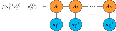
Now you want to find the best MPS that fits the data.

This is a supervised learning problem, it can be solved my minimizing the empirical risk

\[R = \frac{1}{M} \sum^M_{j=1} (f(\mathbf{x}^{(j)}_1 \mathbf{x}^{(j)}_2 \dots \mathbf{x}^{(j)}_N) - y^{(j)})^2\]

over the training dataset.

Following  [3] we now show how DMRG can be employed to minimize \(R\).

DMRG does not try to minimize all the tensors \(A_i\) at once rather it performs forward and backward sweeps along the chain to minimize pairs of tensors.

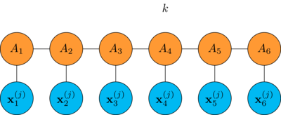
Let's see how it is done for a chain with 6 tensors, first we look at how a single DMRG step is performed

1. pick a position \(k\) in the chain

   

2. merge the tensors \(A_k\) and \(A_{k+1}\) together by contracting the bond between them

   

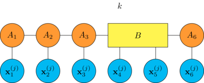
3. compute the gradient of the empirical risk \(R\) with respect to the tensor \(B\)

   \begin{align*} \nabla_B R &= \frac{1}{M} \sum^M_{j=1} \nabla_B (f(\mathbf{x}^{(j)}_1 \mathbf{x}^{(j)}_2 \dots \mathbf{x}^{(j)}_N) - y^{(j)})^2 \\ &= \frac{2}{M} \sum^M_{j=1} (f(\mathbf{x}^{(j)}_1 \mathbf{x}^{(j)}_2 \dots \mathbf{x}^{(j)}_N) - y^{(j)}) \nabla_B f(\mathbf{x}^{(j)}_1 \mathbf{x}^{(j)}_2 \dots \mathbf{x}^{(j)}_N) \end{align*}

   where the gradient \(\nabla_B f\) is

   

   note that \(\nabla_B R\) is a tensor that has the same shape of \(B\)

4. make a stochastic gradient descent step with learning rate \(\lambda\)

   \[B \to B - \lambda \nabla_B R\]

   

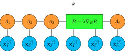
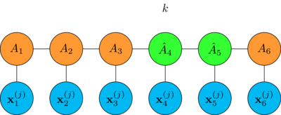
5. finally split the updated tensor by making the singular value decomposition

   \[B - \lambda \nabla_B R = \hat{A}_k \cdot \hat{A}_{k+1}\]

   thus restoring the original MPS shape

   

To optimize the whole chain:

1. sample a mini-batch from the training dataset
2. perform a DMRG step for each pair of tensors from \(k = N-1\) to \(k = 1\) (right to left sweep)
3. at the head of the chain reverse direction and perform the DMRG step moving from \(k = 1\) to \(k = N-1\) (left to right sweep)
4. repeat for a number of epochs

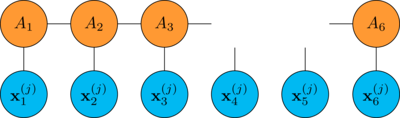
Sweeping like this allows to optimize the computation of the gradient: consider step 3 of the DMRG step, contracting the tensors on the left/right of the "hole" we have

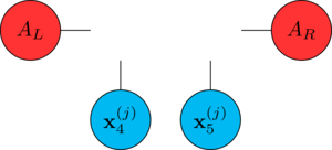
during the sweep, we cache the computation of the contractions \(A_L\) and \(A_R\).

Now you may ask

What's the reason of the merge/split steps? Couldn't we just optimize each tensor in the chain separately?

The merge-optimize-split in the DMRG step achieves two goals at the same time

• to adjust the tensor values
• to tune the MPS bond dimension \(b\)

The DMRG algorithm gradually adapts the total number of the MPS independent parameters to the training dataset increasing the model complexity as needed.

In a sense it is self-regularizing.

By setting a maximum value for the bond dimension or truncating the spectral values in the SVD we can limit the capacity of the model. This can be used to control overfitting.

It's time for an example: let's use DMRG to learn a model of a real function \(f: [0,1] \to \mathbb{R}\) as we did here: pyAutoSpec/Trigonometric Functions.ipynb.

The MPS must be fed a dataset consisting of pairs of a fixed length "word" of p-dimensional vectors and a real number, how do we construct a dataset like this from a function?

We can use the binary expansion of the function argument:

1. fix a length \(N\)
2. generate all the binary words of length \(N\): \(\hat{x} = b_1 b_2 \dots b_N\) (\(b_i \in \{0,1\}\))
3. compute the value of the function \(y = f(x)\) on the value \(x\) whose binary encoding is \(\hat{x}\)

4. take \(\hat{x}\) one-hot encoding

   \[\hat{\mathbf{x}} = \mathbf{b}_1 \mathbf{b}_2 \dots \mathbf{b}_N\]

One-hot encoding consists in the mapping from the alphabet \(\{0,1\}\) to the two dimensional vector space \(\mathbb{R}^2\)

\[0 \to \begin{bmatrix} 1 \\ 0 \end{bmatrix} \hspace{1cm} 1 \to \begin{bmatrix} 0 \\ 1 \end{bmatrix}\]

The resulting dataset now can be used to train the MPS using DMRG. The full implementation can be found here: pyAutoSpec/function mps.py⁴.

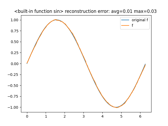
Let's try to learn the sin function in the interval \([0,2\pi]\)

from math import pi, sin
from pyautospec import FunctionMps

sin_mps = FunctionMps(sequence_length=8)
sin_mps.fit(sin, x0=0.0, x1=2*pi, epochs=100, learn_rate=0.1)
sin_mps.comparison_chart()

The comparison with the original function is⁵

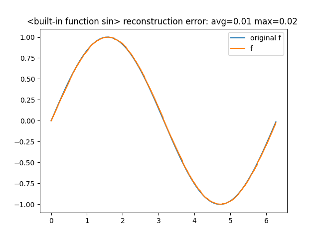
Looking at the bond dimensions

sin_mps.model.bond_dimensions()
# -> [2, 4, 8, 16, 8, 4, 2]

we see that they gradually increase until the middle of the chain then they decrease.

Specifying the max_bond_dim parameter in the constructor we can set a limit to the tensor bond dimensions, effectively reducing the model capacity.

Let's do this and see what happens

sin_mps = FunctionMps(sequence_length=8, max_bond_dim=6)
sin_mps.fit(sin, x0=0.0, x1=2*pi, epochs=100, learn_rate=0.1)
sin_mps.comparison_chart()

the accuracy hasn't changed much, now the bond dimensions are [2, 4, 6, 6, 6, 4, 2].

This and other examples can be found here: pyAutoSpec/Trigonometric Functions (MPS based).ipynb. You can play with different settings and see by yourself how DMRG behave⁶.

Next time we will see DMRG applied to a classification task.