Last time we saw how the DMRG algorithm can be used for learning a MPS. The idea is to sweep forward and backward optimizing the tensors two at a time in order to optimize the bond dimension and by consequence the number of independent parameters.

This is a key property of the DMRG algorithm.

In this post, following  [1], I want to apply DMRG to the task of classification.

Let's get started.

Now, suppose you have a dataset like this

\[\{ (x^{(j)}_1,x^{(j)}_2,\dots,x^{(j)}_N), L^{(j)} \}_{j=1 \dots M}\]

where

• the features are real numbers \(x^{(j)}_i \in \mathbb{R}\)
• the targets are class labels \(L^{(j)} \in \{1,2,\dots,L\}\)

and you want to use a MPS \((A_1,A_2,\dots,A_N)\) as a classifier.

In order to be able to evaluate the MPS over the features we must encode them as vectors. This can be done easily, suppose we have \(x \in [0,1]\) we can encode it as a 2-dimensional vector in this way¹

\[\mathbf{x} = \begin{bmatrix} \cos \frac{\pi}{2} x \\ \sin \frac{\pi}{2} x \end{bmatrix}\]

Also, in order to use the MPS as a classifier, we add an index \(l = 1 \dots L\) (\(L\) is the number of classes) to the last tensor

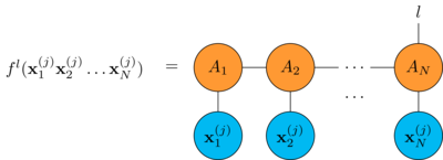
and the predicted label is just

\[\underset{l}{\text{argmax}} f^l(\mathbf{x}_1,\mathbf{x}_2,\dots,\mathbf{x}_N)\]

The empirical risk of the classification problem now is

\[R = \frac{1}{M} \sum^M_{j=1} \sum^L_{l=1} (f^l(\mathbf{x}^{(j)}_1, \mathbf{x}^{(j)}_2, \dots, \mathbf{x}^{(j)}_N) - \delta^l_{L^{(j)}})^2\]

and it can be minimized with the DMRG algorithm as we did last time, the only difference being that now in the merge/split steps we have one more index to take care of. In particular when splitting the tensor \(B\) we have to move the index one place in the direction of the sweep.

All of this is done here: pyAutoSpec/dmrg2 learning.py, pyAutoSpec/mps2.py.

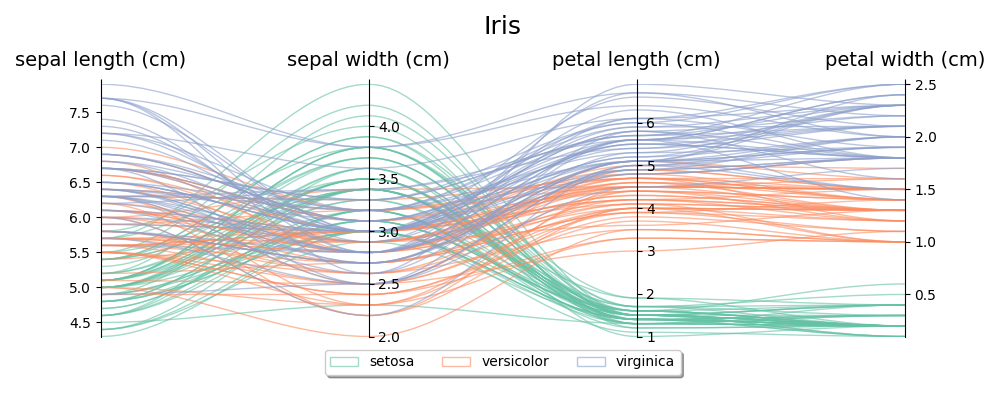
Let's see how it is done in practice, let's take the classic Iris dataset

In order to train a MPS to classify irises we use the DatasetMps class implemented here: pyAutoSpec/dataset mps.py

import numpy as np
from sklearn.datasets import load_iris
from sklearn.model_selection import train_test_split
from pyautospec import DatasetMps

X, y = load_iris(return_X_y=True)
X_train, X_test, y_train, y_test = train_test_split(X, y, test_size=0.3, random_state=42)

iris_mps = DatasetMps(4, class_n=3, x0=np.min(X, axis=0), x1=np.max(X, axis=0), max_bond_d=20)

iris_mps.fit(X_train, y_train, learn_rate=0.05, batch_size=10, epochs = 25)

print(iris_mps)
print("accuracy: {:.2f}%".format(100 * iris_mps.score(X_test, y_test)))

Here we

1. set 30% of the dataset aside for testing
2. initialize an MPS model specifying:
   • the number of tensors (one for each field)
   • the number of classes
   • the minimum/maximum values for the fields
   • the maximum bond dimension
3. fit the model using the training dataset, I do not have specifically optimized the parameters
4. evaluate the model on the test dataset

Running the snippet we get this ascii art output

╭───┐ ╭───┐       ╭─┴─┐
│ 1 ├─┤ 2 ├─ ... ─┤ 4 │
└─┬─┘ └─┬─┘       └─┬─┘

particle dim: 2
   class dim: 3
    bond dim: 6 (max: 20)
        type: classification

accuracy: 100.0%

The accuracy is good, but then this is a trivial example so it was expected.

Inspecting the trained MPS we see that the DMRG algorithm has settled to 6. Lowering it to 4 or even 2 does not change the accuracy significantly.

This is also the case with Wine dataset

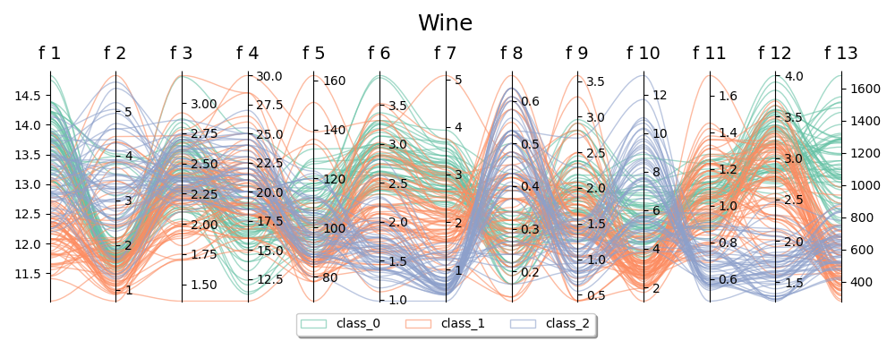
even if it is more complex than Iris (more fields, less obvious patterns) we see that we get high accuracy with a bond dimension of 4.

The Sonar dataset on the other hand is more challenging: we get a 79% accuracy with a bond dimension of 20. Lowering the bond dimension leads to underfitting.

The full code for these examples can be found here: pyAutoSpec/Classification (MPS based).ipynb.

I want to show two more examples:

• the Kaggle Titanic dataset: pyAutoSpec/Titanic Classification (MPS based).ipynb
• the Digits dataset: pyAutoSpec/Digits Classification (MPS based).ipynb

The Titanic dataset is much more challenging than the other examples, first of all because it requires extensive data cleaning, which I didn't do, I mostly copied the excellent work done here: ShauryaBhandari/Kaggle-Titanic-Dataset.

I didn't submit the result to Kaggle, so I don't know the effective performance on the test dataset but the accuracy on the validation dataset is about 80% which is in line with other models.

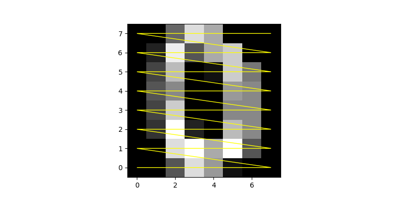
The Digits dataset is an example of how an essentially 1-dimensional MPS model can be used to model 2-dimensional data.

The Digits dataset consists of a collection of 8x8 bitmap images of digits, in order to use them to train a MPS we must convert them into a vector.

This is trivial to do: we concatenate the pixels following a zig-zag path

Then we train the MPS like we have done before. The result is an accuracy of about 95% with a bond dimension of 50.