Automata & Matrix Product States
Looking closely at weighted automata we see that they resemble models used in quantum many body physics.
Take a weighted automata \(A = (\boldsymbol{\alpha}, \mathbf{A}^{(\sigma)}, \boldsymbol{\omega})\) we have seen that it computes a function \(f: \Sigma^\star \to \mathbb{R}\)
\[f(a_1 a_2 \dots a_k) = \boldsymbol{\alpha}^\top \mathbf{A}^{(a_1)} \mathbf{A}^{(a_2)} \cdots \mathbf{A}^{(a_k)} \boldsymbol{\omega}\]
this shape, the product of a chain (or train) of matrices, resembles closely something that is used in quantum physics to deal with the curse of dimensionality in the wave function of a many body system: the matrix product state (MPS).
This analogy has been noted by many authors (for example [1] and [2]) and can be used in many ways:
- on the quantum mechanical side to gain a better insight into the entanglement structure of the wavefunction and to improve the performance of computations
- on the automata theory side to improve the spectral learning algorithm
- algorithms developed by physicist can be repurposed to work with automata
This post is based mainly on [1] and on Guillaume Rabusseau's presentation Tensor Network Models for Structured Data.
As always I want to introduce the minimum of theory that allows to write some code (that you can find here: pyAutoSpec/mps.py) and start experimenting with MPS.
But first of all: what is a tensor?
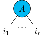
A tensor \(A\) is just a multidimensional array of (real or complex) numbers
\[A_{i_1 \dots i_r} \in \mathbb{R}^{d_1 \times \cdots \times d_r}\]
the number of indexes \(r\) is the rank of \(A\) and each index \(i_n\) has values \(1 \dots d_n\).
A tensor can be represented graphically as a shape with a leg for every index
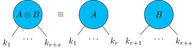
Tensor operations can be represented diagrammatically, for example the tensor product of a rank-\(r\) tensor \(A\) and a rank-\(s\) tensor \(B\) is a rank-\((r+s)\) tensor \(A \otimes B\)
\[[A \otimes B]_{k_1 \dots k_r k_{r+1} \dots k_{r+s}} \equiv A_{k_1 \dots k_r} \cdot B_{k_{r+1} \dots k_{r+s}}\]
and is represented diagrammatically by just drawing \(A\) and \(B\) side to side
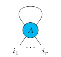
Similarly contracting two indexes \(x,y\) of a rank-\(r\) tensor produces a rank-\((r-2)\) tensor
\[[tr_{x,y} A]_{i_1 \dots i_{x-1} i_{x+1} \dots i_{y-1} i_{y+1} \dots i_r} \equiv \sum_{\alpha=1}^{d_x} A_{i_1 \dots i_{x-1} \alpha i_{x+1} \dots i_{y-1} \alpha i_{y+1} \dots i_r}\]
which is represented by joining the legs corresponding to the contracted indexes
A tensor network is just a diagram containing a bunch of tensors linked together by contraction lines, it can be seen as the graphical counterpart of the Einstein summation convention.
You can look [3] for a comprehensive introduction to the graphical language of tensor networks
These operations can be performed easily in Python1 using NumPy einsum
function:
# make two random 10-dim vectors
u, v = np.random.rand(10), np.random.rand(10)

# tensor product
t_prod = np.einsum("i,j->ij", u, v)
# maps two rank-1 tensors into a rank-2 tensor

# scalar product
s_prod = np.einsum("i,i->", u, v)
# maps two rank-1 tensors into a rank-0 tensor (scalar)
# the repeated index i is contracted

# make a 10x5 and a 5x8 matrix
A, B = np.random.rand(10,5), np.random.rand(5,8)

# their usual product
AB = np.einsum("ij,jk->ik", A, B)
# maps two rank-2 tensors into a rank-2 tensor
# the repeated index j is contracted the other two are carried over
Why tensor networks are so important?
Let's make a brief detour over to quantum mechanics: the first postulate says that (see [4] Ch.2.2)
Any isolated physical system has a state space that is a complex vector space with inner product. The system is completely described by a unit state vector.
the simplest system we can think of is the qubit which has a two-dimensional state space \(\boldsymbol{\psi} \in \mathbb{C}^2\).
Let's now consider \(N\) qubits, another postulate of quantum mechanics says that
The state space of a composite system is the tensor product of the state spaces of the individual subsystems.
thus the state of \(N\) qubits is
\[\boldsymbol{\Psi} \in \mathbb{C}^2 \otimes \mathbb{C}^2 \otimes \cdots \mathbb{C}^2 \equiv \mathbb{C}^{2^N}\]
Fixing a base \(\{\mathbf{e}_i\}\) of the single particle state spaces we can write \(\Psi\) component-wise as
\[\boldsymbol{\Psi} = \sum^2_{i_1 i_2 \dots i_N = 1} \Psi_{i_1,i_2,\dots,i_N} \mathbf{e}_{i_1} \otimes \mathbf{e}_{i_2} \otimes \cdots \otimes \mathbf{e}_{i_N}\]
and its components \(\Psi_{i_1,i_2,\dots,i_N}\) form a rank-N tensor
Now, considering that condensed matter physics deals with systems with \(N \approx 10^{23}\) you see that \(\Psi\)'s space is impossibly huge2.
Clearly we must devise some trick to bring it to reason.
The key observation here is that one is not interested in every possible state but only in the ground state and the low-energy excited states. These are the states relevant for the observable properties of the system.
Approximating \(\Psi\) with a network of small rank tensors would reduce the number of independent parameters.
There are multiple choices3 for the topology of the network. The simplest one is the matrix product state: a chain (or train) of tensors like this
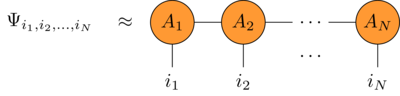
where
- the head \(A_1\) is a \((p \times b)\) rank-2 tensor
- the mid \(A_i\) are \((b \times p \times b)\) rank-3 tensors
- the tail \(A_N\) is a \((b \times p)\) rank-2 tensor
here \(p\) is the dimension of the single particle states (for the qubits \(p = 2\)) and \(b\) is called the bond dimension.
Note that now the matrix product states has only \(O(N b^2 p)\) independent parameters thus we have reduced the space required by \(\Psi\) from exponential to polynomial in the number of particles.
Now, describing quantum states more efficiently is only part of the usefulness of tensor networks, in the words of Orus [5]
.. tensor network techniques offer efficient descriptions of quantum many-body states that are based on the entanglement content of the wave function. Mathematically, the amount and structure of entanglement is a consequence of the chosen network pattern and the number of parameters in the tensors
…
this tensor description offers the natural language to describe quantum states of matter
and that's the big idea: tensor networks reveal the entanglement structure of the quantum state.
I wont'go into entanglement any further in this post. I just want to make the point that, through the tensor network formalism, the concept of entanglement becomes relevant also for automata theory and machine learning.
In Python an MPS can be implemented as a list of tensors (see pyAutoSpec/mps.py)
import numpy as np
mps = [np.random.rand(*s) for s in [(part_d, bond_d)] +
                                   [(bond_d, part_d, bond_d)]*(N-2) +
                                   [(bond_d, part_d)]]
End of the detour, let's go back to WFA.
Looking at the previous MPS it looks very much like a fixed length WFA, let's make the similarity more clear.
First of all let's consider an MPS made of real tensors \((A_1,A_2,\dots,A_N)\) with particle dimension \(p\) and bond dimension \(b\).
Then take \(N\) p-dimensional real vectors \(\mathbf{x}_1, \mathbf{x}_2, \dots \mathbf{x}_N \in \mathbb{R}^p\).
Contracting each \(\mathbf{x}_i\) to the corresponding tensor \(A_i\) we get a scalar
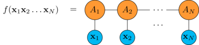
thus the MPS computes a real function from a length \(N\) "word" of vectors to the real numbers.
In Python this can be implemented as
# start contracting the head tensor
T = np.einsum("bp,pj->bj", x[0,:], A[0])
for n in range(1, N-1):
    # contract the middle tensors accumulating the result in T
    T = np.einsum("bi,bp,ipj->bj", T, x[n,:], n)
# finally contract the tail tensor
T = np.einsum("bi,bp,ip->b", T, x[N-1,:], A[N-1])
Now suppose that \(A_i\) in the middle of the chain are all equal4 \(A_i = A\) and the head and tail tensors can be written as \([A_1]_{j,k} = \alpha_i \cdot A_{i,j,k}\) and \([A_N]_{j,k} = A_{j,k,l} \cdot \omega_l\)5.
The resulting MPS is called a uniform matrix product state (uMPS) and can be evaluated on "words" of any length by contracting each \(\mathbf{x}_i\) to the unique \(A\).
So uMPSs are closer than MPSs to WFAs but they are still different: they are evaluated on words made of vectors while WFAs are evaluated on words made of symbols in an alphabet \(\Sigma\).
But it is easy to encode a symbol into a vector: one-hot encoding.
Consider an alphabet \(\Sigma\) with \(L\) letters and fix an order on the letters
\[\Sigma = (a_1, a_2, \dots a_L)\]
then we can encode any letter \(a_i \in \Sigma\) into a L-dimensional vector \(\mathbf{a_i} \in \mathbb{R}^L\) by taking its i-th component as one and the others as zero:
\[\mathbf{a_i}_j = \delta_{i,j}\]
Take an uMPS: it can be extended to words from an alphabet \(\Sigma\) by one-hot encoding, this results in the usual evaluation rule of a WFA.
Let's see how it works in detail: onsider a word \(w = a b c \dots z\) and its one-hot encoding \(\mathbf{w} = \mathbf{a} \mathbf{b} \dots \mathbf{z}\), substituting into the uMPS evaluation rule we get
\begin{align*} f(\mathbf{a} \mathbf{b} \dots \mathbf{z}) &= \alpha_{b_1} A_{b_1,p_1,b_2} a_{p_1} A_{b_2,p_2,b_3} b_{p_2} \cdots A_{b_N,p_N,b_{N+1}} z_{p_N} \omega_{b_{N+1}} \\ &= \alpha_{b_1} A_{b_1,p_1,b_2} \delta_{a,p_1} A_{b_2,p_2,b_3} \delta_{b,p_2} \cdots A_{b_N,p_N,b_{N+1}} \delta_{z,p_N} \omega_{b_{N+1}} \\ &= \alpha_{b_1} A_{b_1,a,b_2} A_{b_2,b,b_3} \cdots A_{b_N,z,b_{N+1}} \omega_{b_{N+1}} \\ &= \boldsymbol{\alpha}^{\top} \mathbf{A}^{(a)} \mathbf{A}^{(b)} \cdots \mathbf{A}^{(z)} \boldsymbol{\omega} \end{align*}which is the usual evaluation rule of a WFA.
In the end we have that: MPS ⊃ uMPS ⊃ WFA
| model | input type | input length |
|---|---|---|
| MPS | p-dim vectors | fixed |
| uMPS | p-dim vectors | variable |
| WFA | symbols in \(\Sigma\) | variable |
Enough, next time we'll see how to learn an MPS.
Footnotes:
there are many
specialized tensor libraries, for example ITensor or Google's TensorNetwork,
but I prefer einsum simplicity for the present purposes
"impossibly huge" here means larger than the number of atoms in the observable universe
going back to quantum mechanics this happens when the system is translationally invariant
repeated indexes are summed over