In the previous post we have started looking at weighted finite automata (WFA), now we would like to use them in real world applications.

Building WFAs by hand is awkward because they are generally non-deterministic and we have to compute the weights ourselves.

But there is another way: we can learn them either from a given function or from some data.

In this post I want to present the spectral learning algorithm introduced by Hsu, Bailly, Balle et al. in the simplest possible terms.

The goal is to build a toy implementation: GitHub - lucamarx/pyAutoSpec to demonstrate spectral learning along with a few applications (function/image compression).

Disclaimer: this post is too short for a complete and accurate account of the math behind spectral learning, I will cover the very bare minimum that allows to write some code. So go read the original papers.

The material of this post is taken from the 2014 paper "Spectral Learning of Weighted Automata"  [1].

Suppose you have a WFA over an alphabet \(\Sigma\)

\[A = (\boldsymbol{\alpha}, \mathbf{A}^{(\sigma)}, \boldsymbol{\omega})\]

that computes a function \(f: \Sigma^\star \to \mathbb{R}\)

\[f(a_1 a_2 \dots a_k) = \boldsymbol{\alpha}^\top \mathbf{A}^{(a_1)} \mathbf{A}^{(a_2)} \cdots \mathbf{A}^{(a_k)} \boldsymbol{\omega}\]

The idea of the spectral learning algorithm is to regard \(f\) as a matrix:

• take \(B \subseteq \Sigma^\star \cup \{\epsilon\}\) as a finite set of words to be used as indexes
• take any two words \(u = u_1 \dots u_m\) and \(v = v_1 \dots v_n\) in \(B\)

• write \(f\) as a \(|B| \times |B|\) matrix in two different ways

  \begin{align*} \mathbf{H}_{u,v} &= f(u_1 \dots u_m v_1 \dots v_n) \\ &= \left[ \boldsymbol{\alpha}^\top \mathbf{A}^{(u_1)} \cdots \mathbf{A}^{(u_m)} \right] \cdot \left[ \mathbf{A}^{(v_1)} \cdots \mathbf{A}^{(v_n)} \boldsymbol{\omega} \right] \\ &= \left[ \mathbf{P} \mathbf{S} \right]_{u,v} \\ \\ \mathbf{H}^{(\sigma)}_{u,v} &= f(u_1 \dots u_m \sigma v_1 \dots v_n) \\ &= \left[ \boldsymbol{\alpha}^\top \mathbf{A}^{(u_1)} \cdots \mathbf{A}^{(u_m)} \right] \cdot \mathbf{A}^{(\sigma)} \cdot \left[ \mathbf{A}^{(v_1)} \cdots \mathbf{A}^{(v_n)} \boldsymbol{\omega} \right] \\ &= \left[ \mathbf{P} \mathbf{A}^{(\sigma)} \mathbf{S} \right]_{u,v} \\ \\ \end{align*}

  note that \(\mathbf{P}_{u,p}\) is a \(|B| \times N\) matrix and \(\mathbf{S}_{q,v}\) is a \(N \times |B|\) matrix where \(N\) is the number of states of \(A\)

• you can then use the Moore–Penrose inverses \(\mathbf{P}^\dagger\) and \(\mathbf{S}^\dagger\) to recover \(\mathbf{A}^{(\sigma)}\) from \(\mathbf{H}^{(\sigma)}\)

  \begin{align*} \mathbf{A}^{(\sigma)} &= \left( \mathbf{P}^\dagger \mathbf{P} \right) \mathbf{A}^{(\sigma)} \left( \mathbf{S} \mathbf{S}^\dagger \right) \\ &= \mathbf{P}^\dagger \left( \mathbf{P} \mathbf{A}^{(\sigma)} \mathbf{S} \right) \mathbf{S}^\dagger \\ &= \mathbf{P}^\dagger \mathbf{H}^{(\sigma)} \mathbf{S}^\dagger \end{align*}

• in order to recover \(\boldsymbol{\alpha}\) and \(\boldsymbol{\omega}\) note that we can define a new vector \(\mathbf{h}\) by taking the row (or column) of \(\mathbf{H}\) with index \(\epsilon\)

  \begin{align*} \mathbf{h}_v &= \mathbf{H}_{\epsilon,v} \\ &= \boldsymbol{\alpha}^\top \cdot \left[ \mathbf{A}^{(v_1)} \cdots \mathbf{A}^{(v_n)} \boldsymbol{\omega} \right] \\ &= \left[ \boldsymbol{\alpha}^\top \mathbf{S} \right]_v \\ \\ \mathbf{h}_u &= \mathbf{H}_{u,\epsilon} \\ &= \left[ \boldsymbol{\alpha}^\top \cdot \mathbf{A}^{(u_1)} \cdots \mathbf{A}^{(u_m)} \right] \boldsymbol{\omega} \\ &= \left[ \mathbf{P} \boldsymbol{\omega} \right]_u \\ \end{align*}

  then, using again the generalized inverses

  \begin{align*} \boldsymbol{\alpha} &= \left( \mathbf{h} \mathbf{S}^\dagger \right)^\top \\ \boldsymbol{\omega} &= \mathbf{P}^\dagger \mathbf{h} \end{align*}

What does all of this have to do with learning?

Of course in a learning problem you don't have an automaton to begin with, but if you can estimate the matrices \(\mathbf{h}\), \(\mathbf{H}\) and \(\mathbf{H}^{(\sigma)}\) then you can compute the WFA \((\boldsymbol{\alpha}, \mathbf{A}^{(\sigma)}, \boldsymbol{\omega})\).

The algorithm goes like this

1. given a finite set of words \(B \subseteq \Sigma^\star \cup \{\epsilon\}\)
2. estimate \(\mathbf{h}\), \(\mathbf{H}\) and \(\mathbf{H}^{(\sigma)}\) from the data
3. find a factorization \(\mathbf{H} = \mathbf{P} \mathbf{S}\)

4. finally compute the WFA

   \begin{align*} \boldsymbol{\alpha} &= \left( \mathbf{h} \cdot \mathbf{S}^\dagger \right)^\top \\ \mathbf{A}^{(\sigma)} &= \mathbf{P}^\dagger \mathbf{H}^{(\sigma)} \mathbf{S}^\dagger \\ \boldsymbol{\omega} &= \mathbf{P}^\dagger \cdot \mathbf{h} \\ \end{align*}

Ok, we are almost at the point where we can write some code, we just need to settle a few details.

First: how do we choose the set \(B\)?

The easiest thing to do is to just enumerate the words from the alphabet \(\Sigma\) up to a fixed length L. In Python we can do

import itertools
# start with the empty word
B = [""]
for l in range(1, L+1):
    # continue by adding all the words of length l
    B.extend(["".join(w) for w in itertools.product(*([alphabet] * l))])

the itertools.product function takes the cartesian product of the list passed as arguments.

Second: how do we estimate \(\mathbf{h}\), \(\mathbf{H}\) and \(\mathbf{H}^{(\sigma)}\)?

Again, to keep things simple, let's suppose that we have a function f that we want our WFA to imitate¹, then we could just compute f for every word in \(B\)

# here we index the elements of both B and the alphabet
B_index        = {B[i]: i for i in range(0, len(B))}
alphabet_index = {alphabet[i]: i for i in range(0, len(alphabet))}
# the loops are over pairs of the word and its index
for (u, u_i) in B_index.items():
    h[u_i] = f(u)
    for (v, v_i) in B_index.items():
        H[u_i, v_i] = f(u + v)
        for (a, a_i) in alphabet_index.items():
            Hsigma[u_i, a_i, v_i] = f(u + a + v)

Third: how do we factor \(\mathbf{H}\)?

We use one of the most widespread techniques in linear algebra: the singular value decomposition. SVD factors the \(|B| \times |B|\) matrix \(\mathbf{H}\) into the product of three matrices:

\[\mathbf{H} = \mathbf{U} \mathbf{D} \mathbf{V}^\top\]

where

• the left singular vectors \(\mathbf{U}\) is a \(|B| \times d\) orthogonal² matrix
• the singular values \(\mathbf{D}\) is a \(d \times d\) diagonal matrix
• the right singular vectors \(\mathbf{V}\) is a \(|B| \times d\) orthogonal matrix

To get more insight about SVD you should read this wonderful introduction³:

Understanding Entanglement With SVD

which explains the SVD factorization in this way

Now, how does this intuition apply to the present situation?

Using linear algebra to understand WFAs forces us to rethink words as vectors instead of strings.

For example taking any word \(u \in B\) we can think of it as a vector in the \(|B|\) dimensional vector space \(\mathbb{R}^{|B|}\)

\[\mathbf{u} = (0,\dots,1,\dots,0)\]

that has zero components except a one at the position of the index of \(u \in B\).

Then if we rewrite \(\mathbf{H}\) elements as

\[\mathbf{H}_{u,v} = \sum_{\alpha,\beta} \left( \sum_i \mathbf{u}_i \mathbf{U}_{i,\alpha} \right) \mathbf{D}_{\alpha,\beta} \left( \sum_j \mathbf{v}_j \mathbf{V}_{j,\beta} \right) = f(uv)\]

we see how it works:

• we take the projection of \(\mathbf{u}\) along each left singular vector \(\mathbf{U}_{:,\alpha}\) (\(\alpha = 1 \dots r\))
• we take the projection of \(\mathbf{v}\) along each right singular vector \(\mathbf{V}_{:,\beta}\) (\(\beta = 1 \dots r\))
• then \(\mathbf{D}\), being diagonal, makes a one-to-one association between the left/right singular vectors (and multiplies the projections by the singular value)

This is then the meaning of "concept":

decomposing a word into a prefix and a suffix (\(w = uv\)) the WFA does not care about the specific prefix/suffix pair, it extract the relevant information (relevant for the calculation of the weight) by projecting them onto the singular vectors (the "concepts")

"Concepts" then are the states: they summarize the features of the input seen so far needed for the calculation of the final weight.

Of course since in general the WFA is non-deterministic a given input may project onto more than one singular vector thus we need to sum over them.

Just one more thing: when performing the SVD decomposition we keep only the \(r < d\) non-zero singular values then we absorb them into the other factors to obtain \(\mathbf{H} = \mathbf{P} \mathbf{S}\).

In Python (using the JAX library) all of this becomes

import jax.numpy as jnp
# compute full-rank factorization H = P·S
U, D, V = jnp.linalg.svd(H)
# truncate expansion
rank = jnp.linalg.matrix_rank(H)
U, D, V = U[:,0:rank], D[0:rank], V[0:rank,:]
# merge singular values
D_sqrt = jnp.sqrt(D)
P = jnp.einsum("ij,j->ij", U, D_sqrt)
S = jnp.einsum("i,ij->ij", D_sqrt, V)

What is remarkable is that even if we have used words up to a length of \(2L+1\) for training, the resulting WFA is valid for words of any length.

The full implementation can be found here: pyAutoSpec/spectral learning.py.

In the previous post we defined a WFA that counted the occurrences of a letter in a word.

How could we learn it? First we define a function that does what we want the WFA to do: count_bs. Then we use the SpectralLearning class to learn it (see pyAutoSpec/Automata Learning.ipynb)

from pyautospec import SpectralLearning
# a function that counts "b"s in a string
def count_bs(s):
    return len([x for x in s if x == "b"])
# create a learner that will use words of length at most L=3
learner = SpectralLearning(["a","b"], 3)
# learn the WFA that counts "b"s
counter = learner.learn(count_bs)

counter is the learned WFA but looking at its diagram⁴

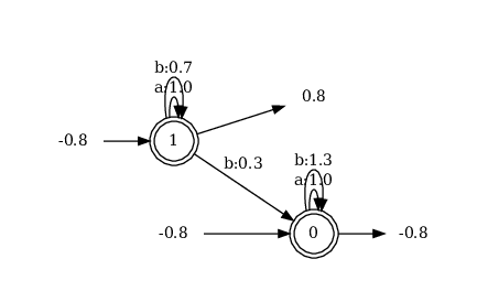
we note that it is different from the one we defined by hand:

• it's true that it has the transition \(1 \xrightarrow{b} 0\) that is responsible for counting "b"s
• but the weights are all different (both on the transitions and on the starting/accepting states)
• and both 0 and 1 are starting and accepting at the same time (in the hand made WFA 1 was starting and 0 was accepting)

despite these differences everything works: if you evaluate counter (for example counter("aaabaa")) you'll see that it effectively counts the number of "b"s in the passed string.

Why is it so?

The fact is that any WFA definition \(A = (\boldsymbol{\alpha}, \mathbf{A}^{(\sigma)}, \boldsymbol{\omega})\) is not unique because we can always take an invertible matrix \(\mathbf{Q}\) and write

and get an equivalent definition \(A = (\boldsymbol{\hat{\alpha}}, \mathbf{\hat{A}}^{(\sigma)}, \boldsymbol{\hat{\omega}})\) with