Using automata to model real functions is a very natural thing to do. For a complete introduction you can look at  [1].

In this post we will use the spectral learning algorithm to build an automaton for a real function and then use it to compute its derivative.

Suppose you have a real function over an interval¹

\[f: [0,1) \to \mathbb{R}\]

can you compute it using a weighted finite automaton (WFA)?

If you could turn \(f\) into a function over words then you could use spectral learning to construct a WFA.

Let's do that: take a number \(x \in [0,1)\), and write it as a binary number

\[x = 0_{\mathbf{2}}.b_1 b_2 b_3 \dots = \sum_{i=1}^\infty b_i 2^{-i}\]

\(b_i\) are binary digits, truncating the expansion to the n-th digit we can represent \(x\) by the word²

\[\hat{x} = b_1 b_2 \dots b_n\]

Now we can convert any function \(f: [0,1) \to \mathbb{R}\) into a function \(\hat{f}: \{0,1\}^\star \to \mathbb{R}\) defined as

\[\hat{f}(\hat{x}) = f(x)\]

In Python this is done like this

def word2real(s : str) -> float:
    s = "0" + s
    return sum([int(s[i]) * 2**(-i) for i in range(0,len(s))])

def real2word(r : float, l : int) -> str:
    if r < 0 or r >= 1:
        raise Exception("out of bounds")
    w = ""
    for _ in range(0,l+1):
        d = 1 if r >= 1 else 0
        w += str(d)
        r = (r-d)*2
    return w[1:]

def f_hat(w : str) -> float:
    return f(word2real(w))

real2word converts a number to its binary (truncated) expansion, while word2real does the opposite conversion.

And that's all, given the function f we can now construct its WFA in this way

from pyautospec import SpectralLearning
learner = SpectralLearning(["0", "1"], 3)
wfa = learner.learn(f_hat)

To use the WFA to evaluate \(f(x)\) you just do this: wfa(real2word(x)).

The full implementation can be found here: pyAutoSpec/function wfa.py.

The FunctionWfa class performs the spectral learning and wraps the resulting WFA in order to make the conversions transparent.

Also it is slightly more general, it allows us to define functions on arbitrary intervals \([a,b)\).

As an example let's try to learn the sin function over \([0,2\pi)\)

from math import sin, pi
from pyautospec import FunctionWfa

sin_wfa = FunctionWfa().fit(sin, x0=0.0, x1=2*pi, learn_resolution=2)

the result is a fairly compact WFA with just 4 states, confronting it with the original function we get

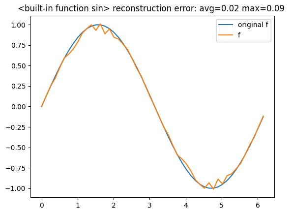
to improve the accuracy it is sufficient to increase learn_resolution to 3, the result now is a slightly larger WFA (6 states) but much more accurate

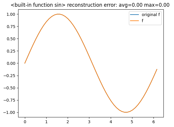
You can find this and other examples here: pyAutoSpec/Trigonometric Functions.ipynb, pyAutoSpec/Polynomials.ipynb.

Now that we have a WFA model of \(f\) is there anything more we can do with it?

How about taking the derivative?

We would like to build a WFA that computes \(f'\) directly from the WFA of \(f\) itself. How would we do it?

First of all the derivative of \(f\) can be approximated as

\[f'(x) \approx \frac{f(x+h) - f(x)}{h}\]

now let's use the same trick we have used earlier: convert \(f': [0,1) \to \mathbb{R}\) into \(\hat{f'}: \{0,1\}^\star \to \mathbb{R}\) by encoding the arguments as their binary expansion

\[\hat{f'}(\hat{x}) = \frac{\hat{f}(\widehat{x+h}) - \hat{f}(\hat{x})}{h}\]

where \(\hat{x} = b_1 b_2 \dots b_n\) corresponds to \(x = 0_\mathbf{0}.b_1 b_2 \dots b_n\).

Now the problem here is \(\widehat{x+h}\), in general it has varying length when changing \(h\) which is inconvenient for us.

So instead of fixing \(h\) we do the other way round, we fix \(\widehat{x+h}\) by just adding a 1 digit to the end of \(\hat{x}\)

\[\widehat{x+h} = \hat{x} \mathbf{1}\]

but now we are left with the task of computing \(h\). This is easily done by subtracting the binary expansions

In the end we have³

\[\hat{f'}(b_1 b_2 \dots b_n) = \frac{\hat{f}(b_1 b_2 \dots b_n \mathbf{1}) - \hat{f}(b_1 b_2 \dots b_n \mathbf{0})}{2^{-(n+1)}}\]

Now we can easily compute the WFA for \(\hat{f'}\), we have:

\[\hat{f}(b_1 b_2 \dots b_n) = \boldsymbol{\alpha}^\top \boldsymbol{A}^{(b_1)} \boldsymbol{A}^{(b_2)} \cdots \boldsymbol{A}^{(b_n)} \boldsymbol{\omega}\]

it follows that

and it's done: the WFA that computes \(\hat{f'}\) is \(A' = (\boldsymbol{\alpha'}, \mathbf{A'}^{(\sigma)}, \boldsymbol{\omega'})\) with

in Python all of this becomes

def wfa_derivative(alpha, A, omega):
  alpha_prime = alpha
  A_prime     = 2 * A
  omega_prime = 2 * jnp.dot(A[:,1,:] - A[:,0,:], omega)
  return (alpha_prime, A_prime, omega_prime)

Again see the full implementation in pyAutoSpec/function wfa.py.

As an example let's consider again the sin function and plot its derivative sin_wfa.prime(x)

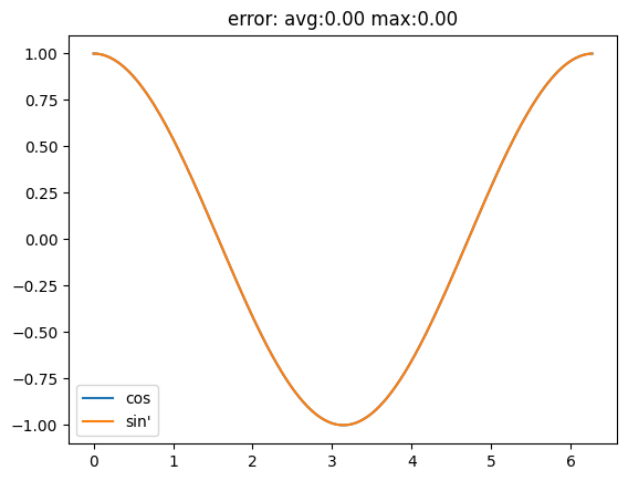
it follows cos quite closely.

This and other examples about derivatives can be found here: pyAutoSpec/Derivative.ipynb.